Active dissociation of intracortical spiking and high gamma activity

Experimental procedures and approval

All procedures were performed under protocols approved by the Northwestern University Institutional Animal Care and Use Committee. Three adult rhesus macaque monkeys were trained in the experimental procedures described below.

Surgery

In each monkey, we surgically implanted a 96-electrode silicon electrode array (Blackrock Microsystems) into M1 contralateral to the arm used to control the cursor. During surgery, monkeys were anaesthetized with isoflurane (2–3%). Anaesthetic depth was assessed at all times by monitoring jaw muscle tone and vital signs. A craniotomy was performed above M1, and the dura was incised and reflected. Electrode arrays were implanted in the proximal arm area, as determined by referencing cortical landmarks and by intraoperative electrical stimulation with a silver ball electrode (2–5 mA, 200-μs pulses at 60 Hz). During stimulation, a reduced level of isoflurane (minimum alveolar concentration lower than 0.5) was supplemented with intravenous remifentanil (0.15–0.30 μg per kg per min) to reduce suppression of cortical excitability. The electrode array was positioned on the crown of the right precentral gyrus, approximately in line with the superior ramus (medial edge) of the arcuate sulcus. The electrode shank length was 1.5 mm. The preamplifier was grounded to the CerePort pedestal and referenced to two platinum wires with 3-mm exposed wire length placed under the dura. A piece of artificial pericardium (Preclude, Gore Medical) was applied above the array, and the dura was closed using 4.0 sutures (Nurolon, Ethicon). Another piece of pericardium was applied over the dura, and the craniotomy partially filled with two-part silicone (Kwik-Cast, World Precision Instruments). The craniotomy was then closed, and the skin was closed. All monkeys were given postoperative analgesics buprenorphine and meloxicam for two and four days, respectively.

Neural signal recording

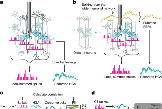
All neural and behavioural data were recorded using a 96-channel Multichannel Acquisition Processor (Plexon). LFP signals were sampled at 1 kHz and band-pass-filtered from 200 Hz to 300 Hz. We deliberately chose this band to be as conservative as possible, because previous studies suggested that components of LFPs above 150 Hz were most contaminated by spike leakage^25,28,29. We computed the spectral power of each electrode from the band-passed LFP by applying a 256-point Hanning window (overlapped by 206 points) and calculating the squared amplitude (power) of the windowed signal’s discrete Fourier transform, yielding 50-ms-binned HGA. Multiunit spikes (threshold crossings) were high-pass-filtered at 300 Hz and sampled at 40 kHz. The signals were further downsampled to 1 kHz. The threshold on each electrode was set at 4.5 s.d. from the root-mean-square baseline activity on the electrode. Note that we also ran a subset of experiments using a lower threshold of 3 s.d. (in the ‘hash’, to reduce the possibility that we were missing some smaller-amplitude spikes near the electrode) and obtained similar results—monkeys could still decorrelate the signals. We defined spikes as unsorted threshold crossings on each electrode. To identify shunted electrodes, we calculated the pairwise R of the spike rates, binned at 1 ms, between all electrode pairs, and removed any electrode that had a pairwise R higher than 0.3 with any other electrodes. For all the analyses except the spike-triggered HGA analysis, we used 50-ms bins for both HGA and spike rates. The above procedures were performed for each file separately. In each file, we also removed electrodes on which the spike rates averaged less than five spikes per second. The available electrodes were used for further analysis after these shunted and low-spike-rate electrodes were removed.

Hand-control task

Three adult rhesus macaques, two male and one female (monkeys C, J and M), used a two-link manipulandum to move a cursor (1-cm-diameter circle) within a rectangular planar workspace (20 cm × 20 cm). The task was a four-target centre–out task, with 2-cm² outer targets spaced at 90° intervals around a circle of radius 10 cm. Each trial began with a target at the centre of the circle. After a random hold time of 0.5–0.6 s within the centre target, a randomly selected outer target was illuminated and the centre target disappeared, signalling the monkey to start a reach. The monkey needed to reach the outer target within 1.5 s and hold for a random amount of time between 0.2 s and 0.4 s to obtain a liquid reward. The task was performed in 10-min files.

ONF task

To maximize monkeys’ ability to control the cursor, we first selected electrodes on which spiking correlated highly with movement during the reach task. First, we computed the absolute value of the Spearman correlation coefficient (|R|) between binned spikes and HGA on each electrode and the velocity in the X and Y directions, respectively, for a total of four correlations (spikes–X, spikes–Y, high gamma–X and high gamma–Y) over a 10-min period. Next, we added the |R| corresponding to X and Y directions for each signal (that is, spikes–X + high gamma–Y; spikes–Y + high gamma–X), giving us two |R| values corresponding to the two possible arrangements of the signals for control. We then selected the electrodes with highest cumulative |R| as inputs (CEs) to use for the ONF task. Later, after monkeys learned to perform ONF control, we selected electrodes that had higher spike–HGA correlations (see below) during hand control.

ONF control was implemented by mapping linear filter outputs of the spike rate and high gamma signals to the X and Y components of cursor velocity, respectively. For either type of signal, we used a linear filter with a set of positive, identical weights set manually on the prior five time bins (50 ms each) of binned spike rates. A bias term was added to the filter output to allow the monkey to reach all parts of the workspace. A dynamic moving mean (averaged over the last 1 min of values) was subtracted from both HGA and spikes before applying filter weights to centre the signals to avoid drift and allow for negative cursor velocity when necessary. Velocity was then integrated to obtain the updated cursor position. Thus, the cursor would have zero velocity when both signals were at their mean activity levels. Both velocity and cursor position signals were computed at 20-Hz resolution.

Initial training involved performing a one-dimensional (1D) BMI task in each of the spike and HG directions. In this case, one 4-cm² target was placed along either the X or the Y axis only, respectively, and the cursor moved directly towards or away from the target. The trials were the same structure as for hand control, except that the hold time was 0.1 s in both centre and outer targets, with a maximum trial time of 15 s for a reward. Trials in which the cursor never reached the target within 15 s or failed to stay in the target for less than 0.1 s were considered failed trials. A typical session (day) lasted approximately 60–90 min (six to nine files), with 10 min (one file) performing hand control and 50–80 min (five to eight files) on BMI control.

Once the number of successes within a file exceeded 40 (typically after 3–7 days), the monkeys were switched to ONF (2D BMI) control. In this case, both filters were applied to their respective signals, and the outputs were mapped to X and Y velocity simultaneously—that is, the cursor moved as a vector sum of filtered spikes and HGA. Targets in this task were the same as in the 1D BMI task, except that they were randomly placed on the X or Y axis in each trial. The rest of the task parameters (hold time, max trial time) were the same as in the 1D task. Because the cursor moved as a vector sum, ONF required the monkeys to increase either spike rate or HGA, while maintaining the other constant, to successfully reach the targets. Target sizes were gradually reduced to operantly condition the monkeys to learn to modulate spike rate and HGA independently. We performed ONF on ten CEs across three monkeys; one was excluded because of noise affecting the spike recordings.

Computing the correlation between spike rate and HGA

To compare the correlation between spike and HGA for each control type (ONF control and hand control), we calculated the Pearson correlation coefficient between single-trial spike rate and HGA of the last second (twenty 50-ms time bins) preceding reward during either ONF control or hand control for every monkey–CE combination. We did this for all trials after the monkeys had become proficient in the ONF task (defined as acquiring at least 40 successes per file). We summarized the distribution of R values for hand control (Fig. 3c, blue) and ONF control (Fig. 3c, red) for every monkey–CE combination.

ONF performance metrics

We measured performance in the ONF task using success rate, time to target, path length, take-off angle and entry angle. We defined success rate as the number of successful trials divided by the total number of trials in each session. We defined time to target as the mean time from the outer target appearance to reward over all trials in each session. We defined path length as the mean cursor path of all the trials in each session. We defined take-off angle as the mode of the distribution of angles formed by the vector of the change in cursor position from 0 to 500 ms after the go cue for all trials in each session. Similarly, we defined entry angle as the mode of the distribution of angles formed by the vector of the change in cursor position in the last 500 ms of the trial for all trials in each session. Take-off and entry angles were further grouped by the target type (spike target versus HG target). To examine whether there were significant changes over sessions and monkey–CE combinations in success rate, path length or time to target, we computed the slopes of the linear fits of the curves of these metrics of every CE across sessions and tested whether the slopes differed from 0 using one-sample t-tests. Similarly, to examine whether the take-off and entry angles converged to 0° (for spike target trials) or to 90° (for HG target trials) over sessions across all monkey–CE combinations, we used one-sample t-tests to test whether the absolute values of the slopes of the fits to these curves were smaller than 0.

DWSS

To examine whether spike leakage from nearby electrodes could explain the HGA during ONF, we computed the DWSS. This assumed that the contribution of spike-related activity to HGA on the CE was inversely proportional to the square of the Euclidean distance between the neuron spiking and the CE⁶¹, and assumed an isotropic medium, which is reasonable within a single cortical layer, which is the case for a Utah array. We calculated the distance-weighted sum of these spike rates (DWSS) from all available electrodes. We considered this sum as a reasonable approximation of the contribution of nearby spike leakage, even with the somewhat sparse sampling of a Utah array, because the listening radius for spikes on an electrode has been estimated^57,58 at 140–200 μm, so most neurons within the plane of the array should be recorded by electrodes spaced apart by 400 μm. This DWSS of CE c was defined as

where fr_n ∈ \({\mathbb{R}}\)^1 × T is the concatenated spike rate of the last 2 s (40 bins) of all successful ONF-control trials recorded on electrode n; T is the number of successful trials \(\times \) 40 bins; d_n is the Euclidean distance between the electrode n and CE; and N is the number of all available electrodes. When n = c, we assumed that the spikes recorded on the CE were from neurons towards the outer part of the listening sphere (d_c = 140 μm, conservative measure⁵⁸) from the recording site, minimizing the impact of the CE spiking on the DWSS.

We then calculated the Pearson’s correlation coefficient between DWSS and HGA of the last 2 s (40 bins) of all concatenated trials on CEs. For CE c, we denote this as: R(DWSS(c),HGA(c)).

To understand the significance of this R value, we compared it to two controls. First, we computed the DWSS for randomly chosen electrodes—each denoted c_random—and calculated its correlation with the HGA of CE c: R(DWSS(c_random),HGA(c)). Second, we calculated the correlation coefficient between DWSS and HGA on that same c_random: R(DWSS(c_random),HGA(c_random)). We performed these calculations for 20 randomly chosen electrodes.

If the value of R(DWSS(c),HGA(c)) were significantly larger than the distribution of R(DWSS(c_random),HGA(c)) across random electrodes, or if it were significantly larger than the distribution of R(DWSS(c_random),HGA(c_random)), it would indicate that the spiking activity on the electrodes near to the CE contributed significantly more to the HGA recorded on the CE than did the spiking activity surrounding a random electrode (Fig. 4g). That is, it would suggest that spike leakage was a significant contributor to HGA.

Factor analysis

To extract the co-firing patterns for every monkey–CE combination, we built a factor analysis model from the z-scored concatenated spike population activity (X ∈ \({\mathbb{R}}\)^N × T) recorded on all available electrodes of all successful ONF–control trials (after ONF proficiency was achieved), where N is the number of electrodes and T is the number of time bins of all concatenated trials. The factor analysis model aimed to explain the correlations of spiking activities among electrodes by assuming they were influenced by common underlying factors (co-firing). Given the number of factors k, X was modelled as X = L × F + R, where L ∈ \({\mathbb{R}}\)^N × k is the co-firing weight, F ∈ \({\mathbb{R}}\)^k × T is the co-firing component and R ∈ \({\mathbb{R}}\)^N × T represents the noise independent to each neuron. The goal was to estimate F and L such that the variance–covariance structure of X was well explained by the common factors, thereby reducing the dimensionality of X while preserving its essential patterns. In Figs. 4h–j and 5, we set k = 1 to extract the most common co-firing component and its corresponding weights. In Fig. 4j, we set k = 1–10 to investigate how the number of factors affected the correlation between the co-firing components and CE spiking or CE HGA. We fitted a linear regression (k = 1) or a multiple linear regression model (k = 2–10) for each k between the trial-concatenated factors and trial-concatenated CE HGA or CE spike rates. We plotted the absolute correlation |R| of these regressions for every monkey–CE combination.

To determine whether the absolute first factor weights |l| ∈ \({\mathbb{R}}\)^N × 1 were significantly higher around the CE than they were around other electrodes, we calculated the distance-weighted mean (DWM) of the absolute factor weights for the CE and for randomly selected electrodes. For electrode e, this is defined as:

where d_n is the Euclidean distance between electrodes n and e. We compared these DWMs (CE versus random) using a one-sided quantile test.

cPCA

We used cPCA to find subspaces in which the monkeys were modulating only HGA or only spikes independently. cPCA found a subspace that maximized variance in the HG+ data (foreground data) and simultaneously minimized variance in the SP+ data (background data)⁶². The same process was used to find SP+-unique components (SP+ cPCs) but using SP+ data as foreground data and HG+ data as background data. cPCs were the eigenvectors of eigenvalue decomposition result on the matrix (C_foreground − αC_background) ∈ \({\mathbb{R}}\)^N × N, where C_foreground ∈ \({\mathbb{R}}\)^N × N and C_background ∈ \({\mathbb{R}}\)^N × N were the covariance matrices of the foreground data and background data, respectively. cPCA has one hyperparameter α, which balances the importance of maximizing variance in the foreground data versus minimizing variance in the background data. An α value of 10 was found to be sufficient to separate SP+ and HG+ data. We chose the top ten cPCs ranked by their row variances for all analyses.

Subspace angle analysis

The principal angles between two subspaces provided a measure of the alignment of those subspaces in a high-dimensional space. These angles were defined recursively, capturing the smallest angles between vectors in the two subspaces. To compute the angles between two m-dimensional subspaces A and B embedded in a high-dimensional neural space spanned by neurons recorded on N electrodes (m < N), we used the method described by Björck and Golub⁶³. We performed singular value decomposition on the inner product of bases W_A ∈ \({\mathbb{R}}\)^N × m and W_B ∈ \({\mathbb{R}}\)^N × m from the m leading PCs (or cPCs) of conditions A and B, respectively:

The principal angles θ_i, i = 1, … , m were the ranked arccosines of the diagonal elements of C.

To assess whether the subspace angles between pairs of subspaces were significantly small, we compared them to the subspace angles between column-shuffled W_A and W_B, which preserved the key statistics of the individual subspace⁶⁴. We used the 0.1th percentile of the distributions of shuffled subspace angles to define a threshold below which angles can be considered significantly small (with a probability P < 0.001).

Spike-triggered average analysis of CE HGA

To determine the relationship between spikes on all available electrodes and CE HGA with high temporal resolution, we used the spike times of all successful trials sampled at 1 kHz to perform spike-triggered average analysis. To compute instantaneous HGA, we used a fourth-order Butterworth band-pass filter at 200–300 Hz bidirectionally on the raw LFP signals sampled at 1 kHz to remove any absolute time delay. Then we applied the Hilbert transform on the filtered signals and squared the amplitude to compute the instantaneous HGA. This method enabled 1-ms resolution in the spike-triggered signal. For any electrode n and its spike event i_n, we first segmented CE HGA from −50 ms to +70 ms relative to the spike time of i_n as HGA(i_n) and averaged these CE HGA segments:

where I is the total number of spikes in the concatenated spiking activity recorded on the electrode n. These spike-triggered average segments were further standardized by their population mean and s.d. We found the argmax of the avgHGA(n) to be the peak time p for any given electrode. Finally, we reported the confidence interval from the distribution of p across all electrodes to be the range of peak time of CE HGA triggered by the electrode.

cPC projection of ONF and hand-control data

To investigate how much the cPCs occupied the spaces spanned by hand-control and ONF-control data, we projected the hand-control data and ONF data onto different cPCs. First, we concatenated the trials of population spiking activity during hand control and ONF control \({{\bf{X}}}_{{\rm{c}}{\rm{t}}{\rm{r}}{\rm{l}}}\in {{\mathbb{R}}}^{N\times {j}_{{\rm{c}}{\rm{t}}{\rm{r}}{\rm{l}}}}\) separately, where ‘ctrl’ is either hand-control or ONF-control type and j_ctrl represents the length of concatenated trials of that control type, respectively. Then, we projected the z-scored X_ctrl into the cPC space to obtain the m-dimensional latent \({{\bf{Z}}}_{{\rm{c}}{\rm{t}}{\rm{r}}{\rm{l}}}^{{\rm{c}}{\rm{o}}{\rm{n}}{\rm{d}}}\in {{\mathbb{R}}}^{{j}_{{\rm{c}}{\rm{t}}{\rm{r}}{\rm{l}}}\times m}\): \({{\bf{Z}}}_{{\rm{c}}{\rm{t}}{\rm{r}}{\rm{l}}}^{{\rm{c}}{\rm{o}}{\rm{n}}{\rm{d}}}={{\bf{X}}}_{{\rm{c}}{\rm{t}}{\rm{r}}{\rm{l}}}^{T}{{\bf{W}}}_{{\rm{c}}{\rm{o}}{\rm{n}}{\rm{d}}},\) where ‘cond’ represents the spike–HG angle of either HG+ or SP+, and \({{\bf{W}}}_{{\rm{c}}{\rm{o}}{\rm{n}}{\rm{d}}}\in {{\mathbb{R}}}^{N\times m}\) represents the m-dimensional space provided by the m leading cPCs. Finally, we calculated the variance accounted for (VAF) for each cPC dimension \({{\bf{Z}}}_{{\rm{c}}{\rm{t}}{\rm{r}}{\rm{l}}}^{{\rm{c}}{\rm{o}}{\rm{n}}{\rm{d}}}\): \({\rm{V}}{\rm{A}}{\rm{F}}({{\bf{Z}}}_{{\rm{c}}{\rm{t}}{\rm{r}}{\rm{l}}}^{{\rm{c}}{\rm{o}}{\rm{n}}{\rm{d}}})=\frac{{\rm{c}}{\rm{o}}{\rm{l}}{\rm{v}}{\rm{a}}{\rm{r}}\left({{\bf{Z}}}_{{\rm{c}}{\rm{t}}{\rm{r}}{\rm{l}}}^{{\rm{c}}{\rm{o}}{\rm{n}}{\rm{d}}}\right)}{{\rm{v}}{\rm{a}}{\rm{r}}({{\bf{X}}}_{{\rm{c}}{\rm{t}}{\rm{r}}{\rm{l}}})},\) where colvar(*) represents the variance calculation along the matrix column (cPC dimension) and var(*) represents the total variance calculated on the flattened matrix (the asterisk (*) represents any possible value of the variable). We calculated the VAF for every ctrl–cond combination. For example, when ctrl was ONF control and cond was SP+, VAF was calculated on the trial-concatenated ONF-control data projected into SP+ cPC space.

Reporting summary

Further information on research design is available in the Nature Portfolio Reporting Summary linked to this article.